How Fast Can We Plan It?
Single-Shot Neural Motion Planner

Abstract

We present a single-shot neural motion planner that maps a compact scene context and a 2D occupancy map to a small set of trajectory breakpoints (times and joint states) and a feasibility score in one forward pass. Trained on RRT-Connect demonstrations compressed with Ramer–Douglas–Peucker (RDP) and refined with collision-aware fine-tuning, the planner delivers single-digit millisecond CPU latency with far lower variance than classical tree-based planners. In a ball-drop interception benchmark it yields a smaller critical height, reallocating precious time from planning to execution.

Demo Videos

Key Contributions

• Single-shot, scene-wide prediction of an entire trajectory as a compact set of breakpoints, replacing incremental explore-and-extend.
• Compact supervision via RDP-simplified expert paths; the model learns structural primitives (breakpoints) instead of dense waypoints.
• Three-head design (feasibility, timing, states) with goal and smoothness terms, plus collision-aware fine-tuning.
• New time-critical benchmark (ball-drop) and spatial planning-time maps showing lower, more uniform latency than RRT-Connect.

Background: RRT-Connect and RDP

RRT-Connect grows two trees using a straight-line local planner, yielding a path that is inherently piecewise-linear in configuration space. After time-parameterization, many waypoints are redundant. We compress each expert path with the RDP algorithm, which recursively removes points whose orthogonal deviation to a segment is below a tolerance, keeping only breakpoints that preserve geometry. This shrinks hundreds of waypoints to a handful of key poses and times, simplifying supervision and speeding learning.

Figure: RDP compresses a dense RRT-Connect trajectory into a compact sequence of breakpoints.

Method

Planner Overview

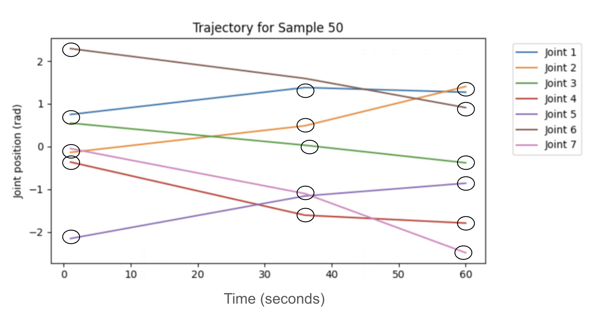
We cast motion generation as a single-shot mapping from scene context (start, goal, and obstacle descriptors) and a 2D occupancy map to a compact trajectory in joint space. The network predicts a sequence of N breakpoints {(ti, θi)} for a 7-DoF arm, plus a feasibility score; planning is performed in a single forward pass rather than by incremental search. Because RRT-Connect paths are polylines, a small set of breakpoints suffices to reconstruct the motion, and a CNN can “see” the full environment at once, making latency less sensitive to scene scale.

Context CNN

Context encodes task and scene parameters—start state, goal state, and obstacle attributes (size, position, orientation). A Conv2D → BatchNorm → ReLU stem, followed by four residual blocks, transforms this structured input into a fixed-width context embedding that captures interactions among start/goal and obstacle terms.

Map CNN

The Map CNN ingests a 64×64×C occupancy grid (optionally with distance fields or inflated obstacles) and can concatenate normalized coordinate channels (CoordConv) to ease learning of absolute position. A Conv–BN–ReLU stem leads into residual stages with stride-2 downsampling (32→64→128 channels), optionally using dilated 3×3 kernels for long-range context. Global average pooling yields the map embedding, followed by dropout.

Output Heads

Fusing the context and map embeddings, a small MLP produces three heads: (i) feasibility, a sigmoid probability used with binary cross-entropy; (ii) timing, positive increments accumulated via softplus and cumsum to form breakpoint times with a stop token; and (iii) joint states, either absolute or residual, recovered via cumulative summation. The breakpoints are linearly interpolated and then time-parameterized to satisfy limits.

Loss and Collision-Aware Fine-Tuning

The training objective is a weighted sum of feasibility (BCE), timing and state accuracy (Huber), goal-consistency, and smoothness on first/second differences. After pretraining, we fine-tune with a clearance penalty that pushes configurations away from obstacles using a hinge on signed distance (from a distance field or proximity query). This retains timing/goal accuracy while reducing residual contacts, and gradients flow through the differentiable distance surrogate.

Data Collection

We generate randomized scenes by sampling obstacles and valid start/goal states for a 7-DoF Panda, plan with OMPL’s RRT-Connect subject to a timeout, label infeasible scenes accordingly, and compress successful paths with RDP to obtain breakpoint sequences and timestamps. We rasterize each scene into a 2D occupancy grid and store (context, map, simplified breakpoints, feasibility). The dataset comprises 100k samples (80k/20k train/val).

Experiments

Planning Time

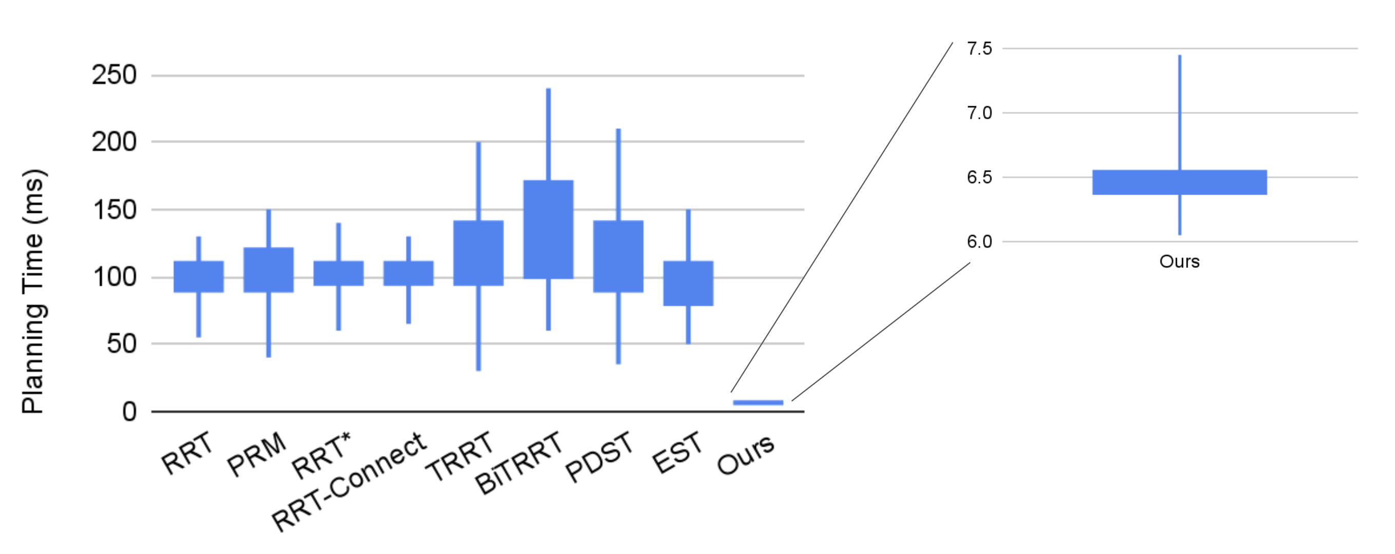
Boxplots show that classical planners (RRT, PRM, RRT*, RRT-Connect, EST, etc.) have medians around 95–115 ms with wide tails; heuristic variants (TRRT, BiTRRT, PDST) are typically slower and more variable. Our single-shot planner is tightly concentrated near ≈6.4 ms with whiskers within 6.0–7.5 ms, a 15–26× reduction in median latency and dramatically smaller dispersion.

Planning-time distribution across planners (zoomed inset shows our method).

Ball-Drop Interception

In a drop-and-intercept test, available reaction time scales as t = √(2h/g). Because our plans arrive in single-digit milliseconds and with low variance, the system succeeds at smaller critical heights than RRT-Connect—freeing more of the reaction window for execution and improving reliability in time-critical settings.

Spatial Dependence

Mapping goals on concentric circles around home produces spatial planning-time maps. RRT-Connect shows pronounced spatial nonuniformity as latency depends on where exploration encounters obstacles. Our single-shot planner, which reasons over the full map at once, exhibits both lower and more uniform times across space, crucial for predictable control budgets.

Limitations

The model is trained on static 2D occupancy grids; out-of-distribution geometry, fine 3D effects, or moving obstacles can degrade reliability. It lacks probabilistic completeness/optimality guarantees and relies on post-hoc time-parameterization for limits. RDP-compressed supervision can bias toward straighter polylines, and the clearance surrogate used in fine-tuning approximates geometry. A fixed breakpoint budget constrains very long motions, and porting to new robots/workspaces generally requires new data and retraining. Finally, system-level responsiveness also depends on perception and control latencies.

Conclusion & Future Work

We reframed planning as perception and demonstrated a CPU-fast single-shot planner with compact breakpoint outputs, RDP-based supervision, and collision-aware fine-tuning. It achieves consistently lower latency than classical baselines and improves time-critical success in a ball-drop test. Future work targets dynamic scenes and receding-horizon updates, richer geometric encodings and end-to-end perception-to-plan, integrated kinodynamic constraints and safety certificates, scaling via stronger data/continual learning, and a real-time ROS 2/MoveIt 2 deployment.