← sakibchowdhury131.github.io

Learning to Strike for Robotic Table Tennis

Sakib Chowdhury  ·  Yi Guo
Department of Electrical and Computer Engineering, Stevens Institute of Technology
Paper (PDF) BibTeX
Simulated table-tennis strikes and ball interception, played back at 1× speed in PyBullet.

Abstract

Motivated by recent advances in robotic systems’ ability to interact with dynamic environments, we study autonomous robotic table tennis in this paper. We design a high speed robotic arm to play table tennis, and develop a software system that predicts the incoming ball’s trajectory and learns to control the robot arm for striking the ball to the opponent side of the table. Utilizing the idea of residual physics, we develop a residual predictor to predict a striking position for the incoming ball using sparse observation of the ball’s starting trajectory. We control the arm to the contact-ready position, and then use a neural network to output the striking velocity to hit the ball. The neural network is trained through experience using a regression-based learning method. Simulation results in a robotic simulator demonstrate the superior performance, benefiting from efficient learning.

Highlights

The System & Problem

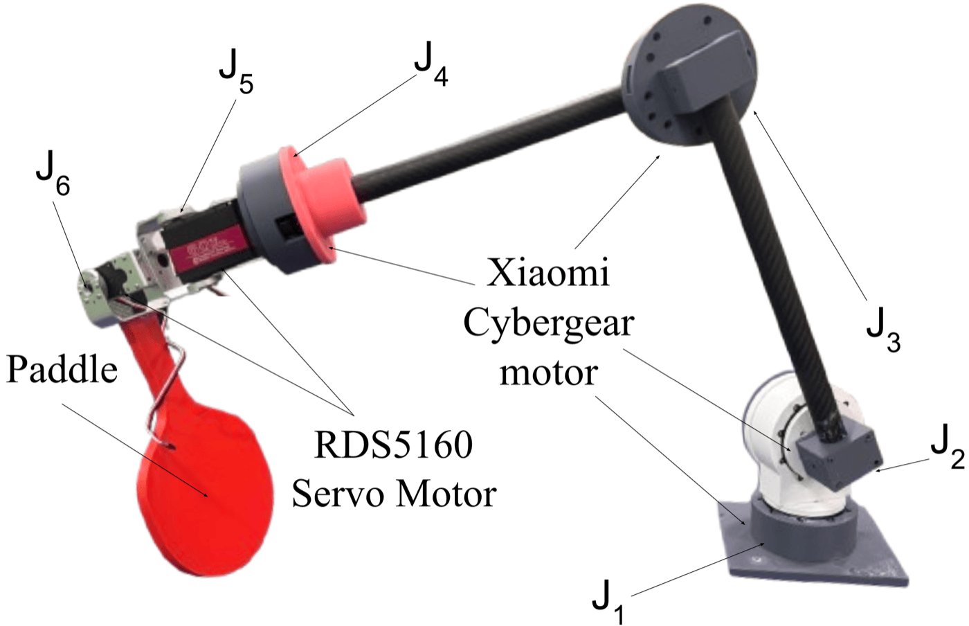
Commercial robotic arms are designed for safe, limited-speed operation, making most of them unsuitable for table tennis. We therefore design a custom 6-DOF arm: joints J1–J4 use Xiaomi Cybergear motors (continuous rotation, up to 296 rpm, 12 N·m peak torque), while J5 and J6 use RDS5160 servos (0–270°, up to 461°/s, 6.87 N·m peak torque) placed along the paddle’s roll, pitch, and yaw axes for precise orientation control.

Design of the custom 6-DOF robotic arm, showing the Xiaomi Cybergear motors, RDS5160 servo motors, and paddle end-effector
Fig. 1 — The custom high-speed 6-DOF arm. J1–J4 use Xiaomi Cybergear motors; J5–J6 use RDS5160 servos and are aligned with the paddle’s roll/pitch/yaw for precise orientation.

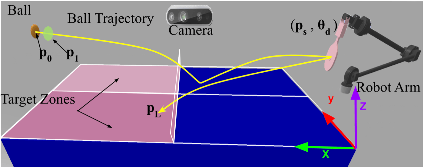
Given the first two camera-observed positions of a thrown ball, p0 and p1, the goal is to compute joint angular velocities that strike the ball so it lands at a desired location pL on the opponent’s side — with the striking point ps constrained to a fixed plane in front of the robot, and a pre-strike paddle orientation θd.

Setup diagram: a camera observes the ball's early trajectory, the robot arm strikes it toward target zones on the opponent's side of the table
Fig. 2 — The table tennis setup. A camera observes the ball’s first two positions p0, p1; the robot strikes the ball toward a target landing position pL in the opponent’s target zones.

Method

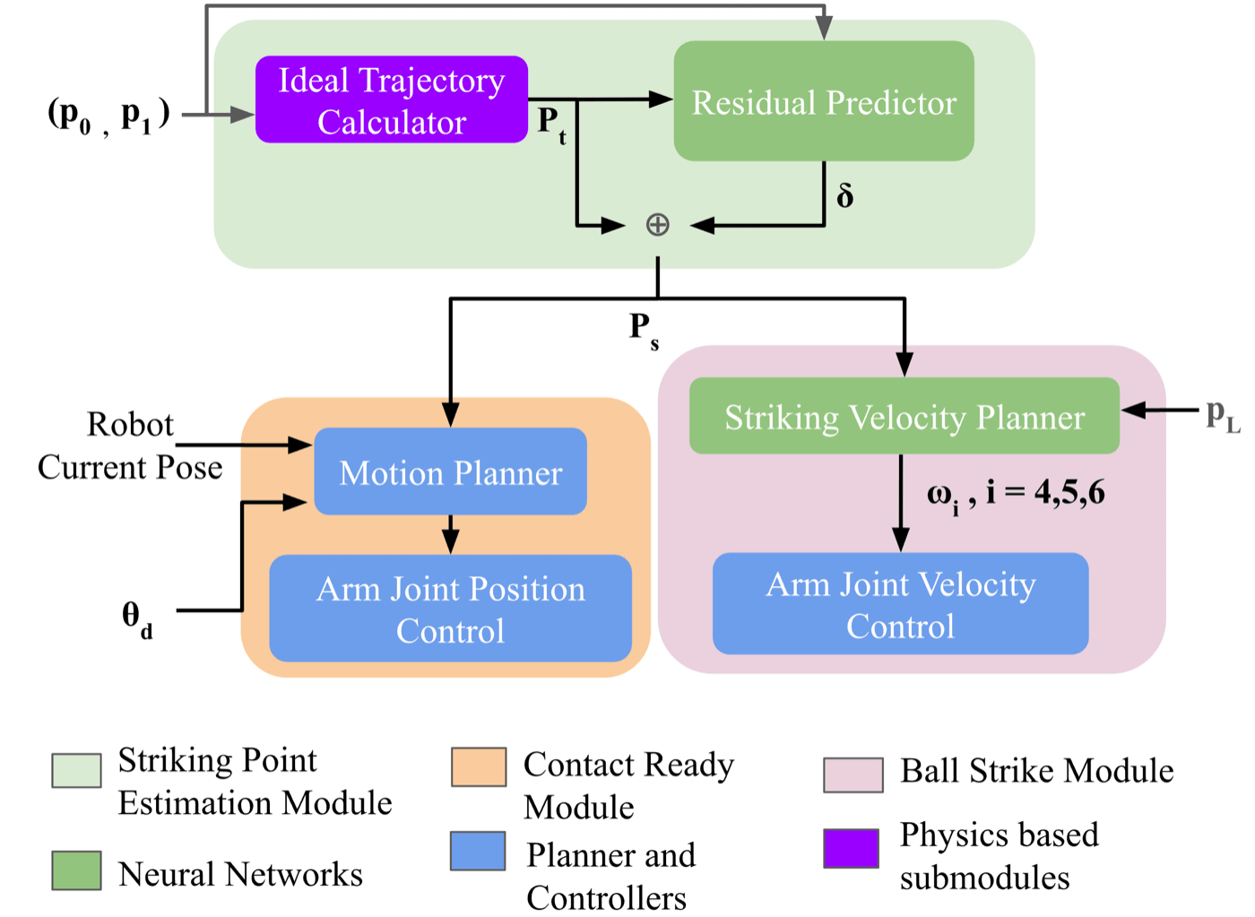
The system has three modules: a Striking Point Estimation module predicts where to intercept the ball, a Contact Ready module moves the paddle there, and a Ball Strike module predicts the joint velocities needed to hit it toward the desired landing spot.

System architecture: striking point estimation module, contact ready module, and ball strike module, with physics-based and neural-network submodules
Fig. 3 — System architecture. The physics-based ideal trajectory (purple) is corrected by a learned residual (green) to estimate the striking point ps, which feeds a motion planner (orange) and a learned striking-velocity planner (pink).

Striking Point Estimation: Residual Learning

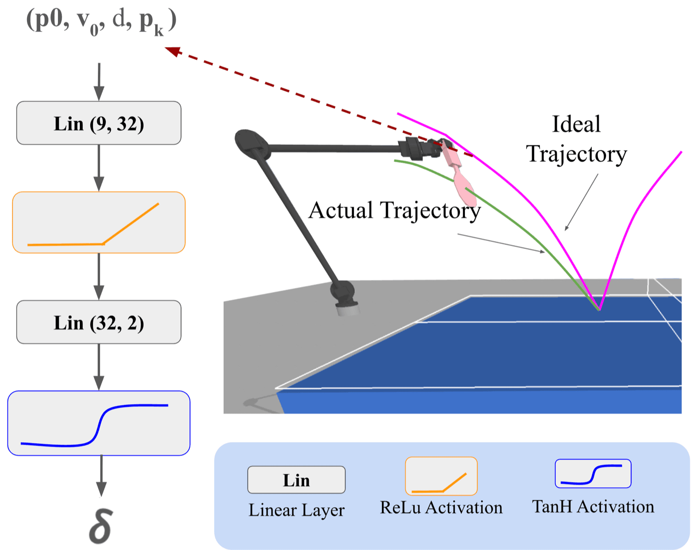
From p0 and p1, an initial velocity v0 gives an ideal projectile-motion trajectory Pt. But real trajectories deviate from this ideal due to the table’s coefficient of restitution, friction, and air resistance — effects that are hard to model explicitly. Rather than modeling them, we learn the deviation δ directly: a shallow feedforward network (two linear layers, ReLU then TanH) takes p0, v0, the distance to the robot, and the ideal striking point pk, and predicts δ, so the actual striking point is ps = Pt + δ. The shallow architecture keeps inference to about 4.3 ms.

Residual predictor architecture (two linear layers with ReLU and TanH activations) and an illustration of the ideal versus actual ball trajectory
Fig. 4 — The residual predictor: a two-layer network mapping (p0, v0, d, pk) to the residual δ between the ideal (magenta) and actual (green) trajectory.

Contact Ready & Motion Planning

Once ps and the pre-strike orientation θd are known, an RRT-Connect motion planner computes the joint trajectory that brings the paddle from its current pose to the target pose, executed by the arm’s joint position controller.

Ball Strike: Learning the Striking Velocity

With the paddle positioned at ps, the joint velocities ω4, ω5, ω6 (roll/pitch/yaw — sufficient to direct the ball anywhere) are predicted as a function of v0, ps, and the desired landing position pL. We model this mapping with a random forest regressor, trained on data collected by hitting the ball with random joint velocities and recording where it lands; a PID controller then executes the predicted velocities at the moment of contact.

Results

Validated in a PyBullet simulation matching standard table tennis dimensions and ball properties (20 mm radius, 2.7 g), with a restitution coefficient of 0.75 and modeled table friction and air resistance.

Residual Predictor

Across 1000 thrown-ball trials, the residual predictor outperforms every baseline regressor tested on MSE, MAE, and R2 for estimating δ.

ModelMSE (y)MAE (y)R² (y)MSE (z)MAE (z)R² (z)
SVR0.00110.0274−4.290.00690.06830.775
Decision Tree0.00040.0074−0.940.00690.04830.777
Random Forest (20)0.000230.00688−0.050.004090.03870.869
KNN0.00020.0061−0.330.00510.04750.835
Ours0.00010.00530.1990.00410.03460.888

The Y-axis R2 is comparatively modest, but the residual there is small in absolute terms next to the Z-axis residual — qualitatively, our model still reliably locates the collision point.

Motion Planning

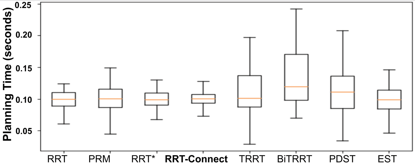
Among eight classical motion planners benchmarked over 1000 random target points, RRT-Connect had both the lowest mean planning time and the tightest interquartile range, motivating its use in the contact-ready module.
Boxplot of planning times for RRT, PRM, RRT*, RRT-Connect, TRRT, BiTRRT, PDST, and EST
Fig. 5 — Planning time comparison across motion planners; RRT-Connect (bold) offers the most consistent, lowest planning time.

Striking Velocity Planner

Repeating the striking-velocity experiment 1000 times with varied throw velocities and target landing positions, the Random Forest regressor with 160 estimators achieved the best R2 across all three rotation axes tested.

ModelRollPitchYaw
MAEMSEMAEMSEMAEMSE
Decision Tree0.6812.4920.30.7024.2738.50.1692.138.06
KNN0.7962.3213.00.6524.3345.00.6621.373.27
SVR0.8002.7012.70.6654.1543.30.5961.523.92
Random Forest (160, ours)0.8871.547.210.6894.3340.20.6871.353.04
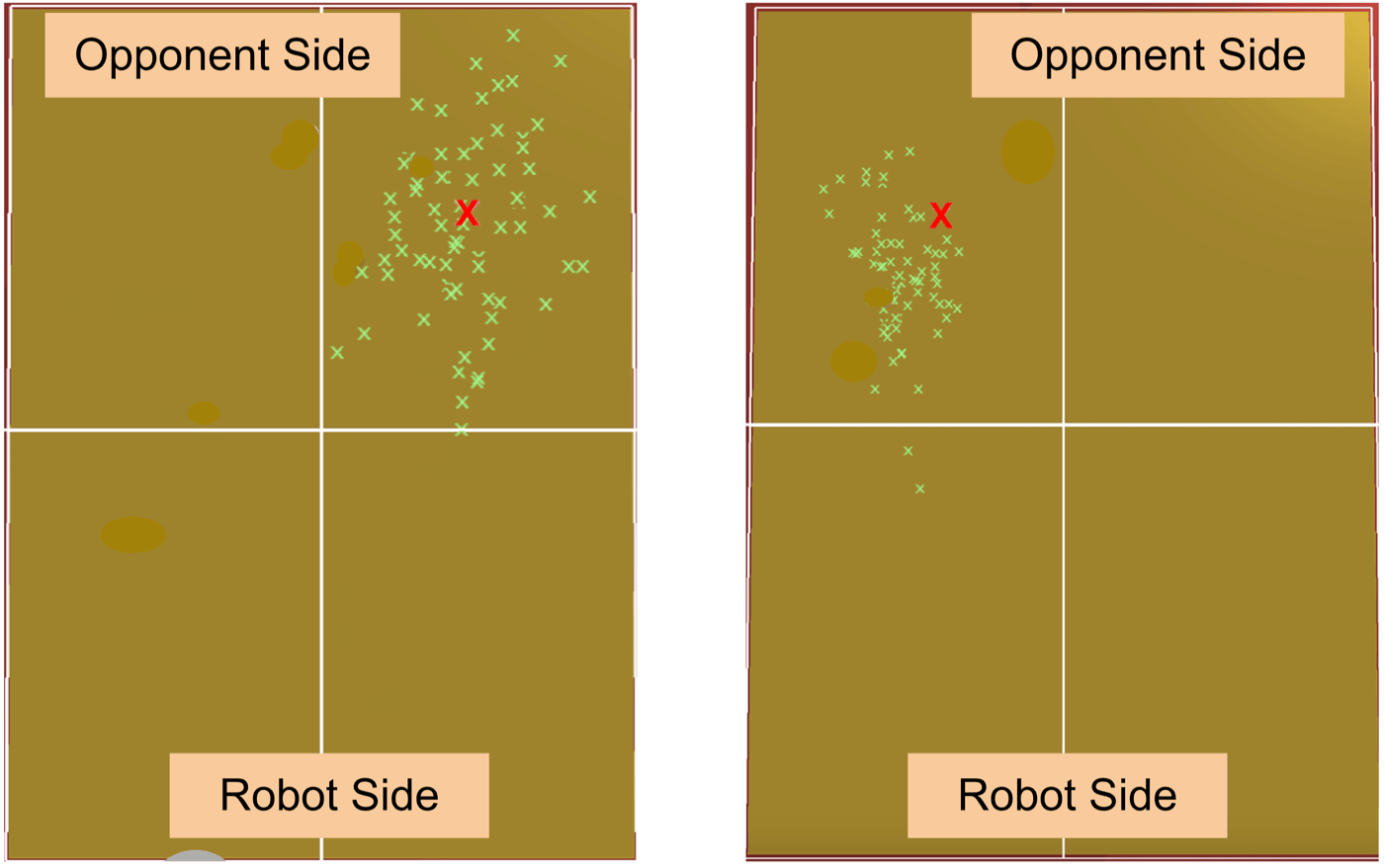
Two example target zones showing intended hitting point (red X) and where the ball actually landed across trials (green X marks clustered nearby)
Fig. 6 — Qualitative accuracy of the striking velocity planner: intended target (red ×) versus actual landing positions (green ×) across repeated trials.

End-to-End Performance

Across 1000 randomly thrown balls, the full system — residual predictor plus learned striking velocity — successfully intercepted 985, a 98.5% success rate. Without the residual predictor, relying on the physics-only trajectory alone, the system consistently failed to intercept the ball, since each bounce alters the trajectory in ways the ideal model cannot capture.
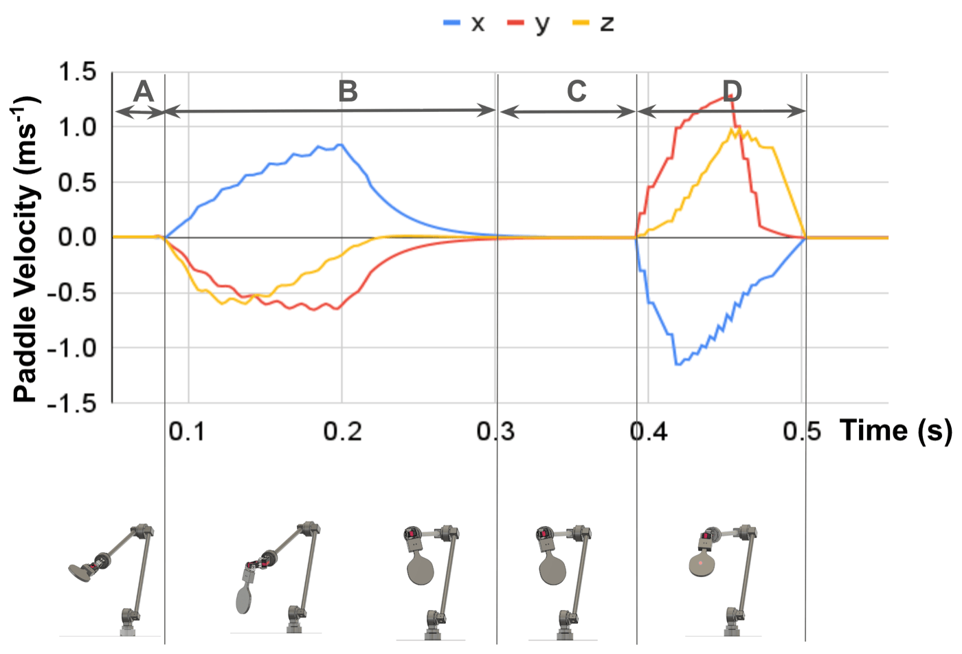
Paddle velocity over the four operational stages A (estimate/plan), B (move to contact-ready), C (wait for ball), D (execute strike), with corresponding arm poses below
Fig. 7 — Paddle velocity across the four operational stages: (A) estimate the striking point and plan, (B) move to the contact-ready pose, (C) wait for the ball, (D) execute the learned strike.
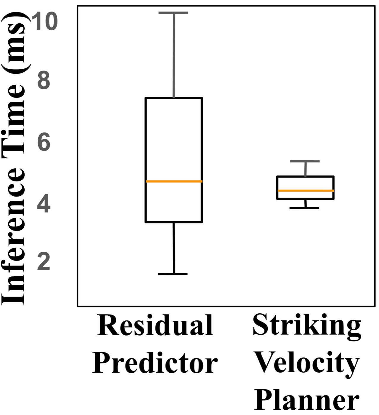
Boxplot of inference times for the residual predictor (median 4.3ms) and the striking velocity planner (median 4.2ms)
Fig. 8 — Inference times: the residual predictor (median 4.3 ms) and striking velocity planner (median 4.2 ms) together add well under 16 ms, leaving ample budget for motion planning and control.
Limitations & Future Work

This work validates the approach entirely in a PyBullet simulation, assuming the first two ball positions come from an upstream perception system; a real robot experiment is beyond the current paper’s scope. Future work includes integrating a high-speed 3D perception system for real-time ball tracking on the physical arm, building a real-time control stack for low-latency contact-ready and strike execution, adapting the striking-point estimator to real sensor noise, and fine-tuning motion planning and control for the hardware’s constraints.

Conclusion

We presented a learning-from-demonstration approach to robotic table tennis built from three modules: striking point estimation, contact-ready motion, and ball striking. A residual learning scheme corrects a physics-based trajectory estimate using only the ball’s first two observed positions, and a random forest regressor learns the striking velocity needed to direct the ball to a target landing position. Compared to reinforcement-learning approaches that require extensive, potentially unsafe real-world trial-and-error, this sample-efficient formulation reaches 98.5% interception success in simulation while keeping both learned components fast enough — a few milliseconds each — for real-time play.

Citation

This paper is currently under review. If you’d like to reference it in the meantime:

@misc{chowdhury2025learningtostrike,
  title  = {Learning to Strike for Robotic Table Tennis},
  author = {Chowdhury, Sakib and Guo, Yi},
  note   = {Submitted, under review},
  year   = {2025}
}