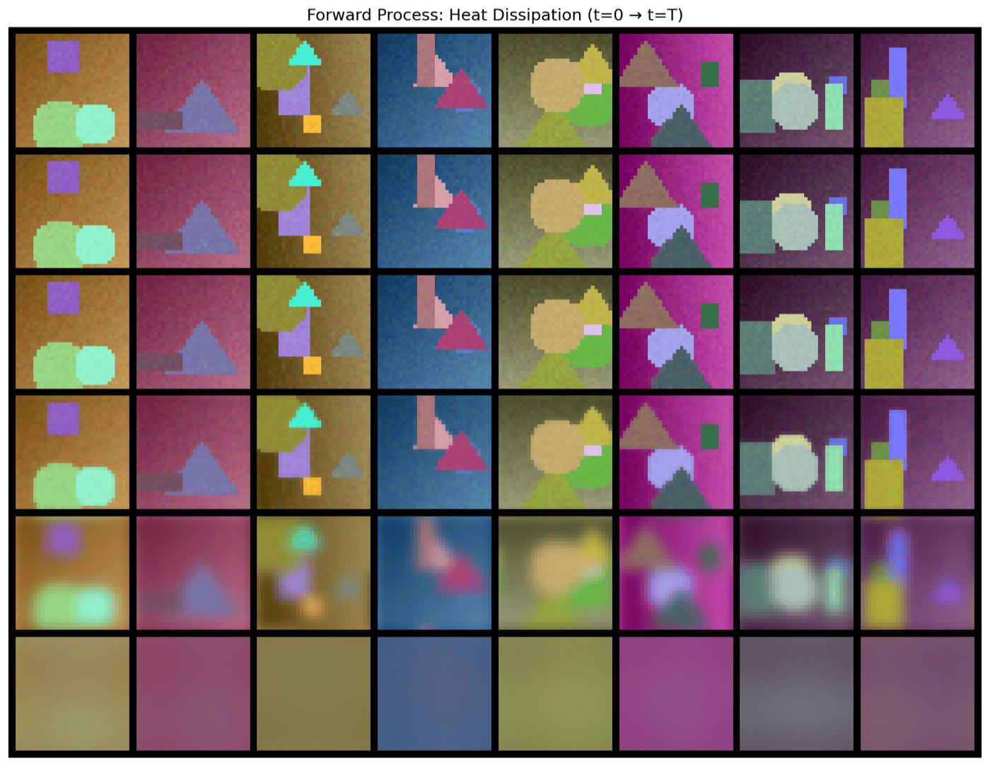
Heat Dissipation Image Generation: Diffusion by Reversing the Heat Equation

Replacing Gaussian Noise With the Heat Equation

Standard diffusion models corrupt an image with independent Gaussian noise at every pixel, destroying every spatial frequency at the same rate. The heat equation corrupts an image differently: it is equivalent to convolving with a Gaussian kernel whose width grows with time, which in frequency space is a low-pass filter that gets progressively narrower. High-frequency detail (edges, texture) is attenuated fastest; low-frequency structure (overall color, rough shape) survives the longest. Run forward far enough, and any image converges to a single flat field — not to random noise.

clean image u₀—heat blur→flat field u_T

u_tmodel predictsû₀—re-blur to t−1→u_t−1

Forward heat dissipation process applied to synthetic shape images across increasing blur levels, converging to a flat field

Eight sample images (columns) blurred at six increasing timesteps (rows, top to bottom). By the last row, every image has converged to a near-uniform flat color — the deterministic endpoint the heat equation always reaches.

Aspect	Standard diffusion	Heat dissipation (this work)
Forward corruption	add i.i.d. Gaussian noise	blur with the heat kernel (FFT multiply)
Frequency treatment	every frequency corrupted equally	high frequencies die first, low frequencies survive longest
Network predicts	`noise ε, then u0 = ut − ε`	`clean image u0 directly`
Mass conservation	not applicable	exact — the zero-frequency (mean color) term is untouched by construction
Endpoint at t=T	pure random noise	a deterministic flat field (the image's own average color)

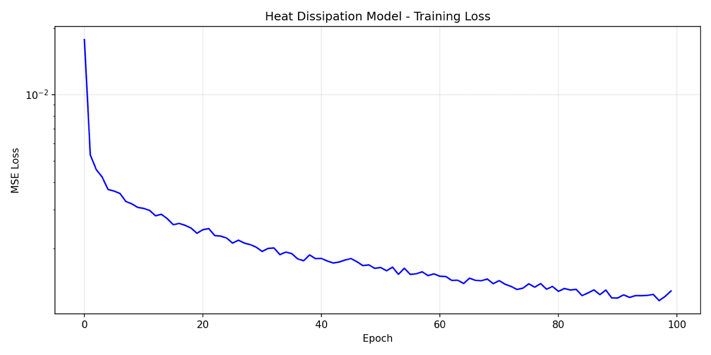
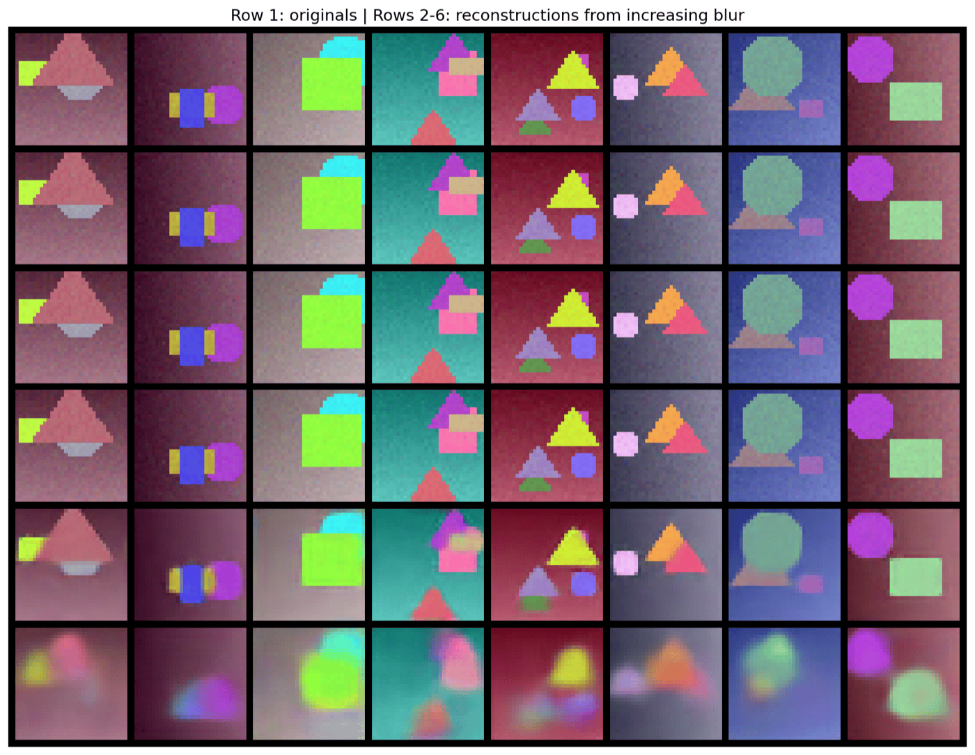
A U-Net That Predicts the Clean Image, Not the Noise

A time-conditioned U-Net f_θ(u_t, t) takes the blurred image and a sinusoidal embedding of the blur level t, and predicts the original clean image u₀ directly — unlike standard diffusion policies, which predict the noise that was added and subtract it out. The network uses residual blocks with GroupNorm and time-conditioning at every stage, encoder/decoder skip connections, and is trained with a single MSE loss between the prediction and the ground-truth image at a randomly sampled blur level per batch.

Setting	Value
Dataset	5,000 synthetic 32×32 images — geometric shapes with gradient backgrounds
Model size	6,231,363 parameters
Blur schedule	30 timesteps, log-spaced σ from 0.01 to 10
Optimizer	AdamW, lr 2e-4, cosine annealed, gradient-clipped at 1.0
Training	100 epochs, batch size 64
Loss	MSE between predicted and ground-truth clean image

Training loss curve over 100 epochs on a log scale, decreasing from about 0.018 to 0.0013

MSE loss (log scale) over 100 epochs: 0.0178 → 0.0013, a smooth and fully converged descent with no instability — despite each batch seeing a different randomly sampled blur level.

Reconstruction: Recovering a Real Image From Its Blurred Version

The most direct test of f_θ is reconstruction: take a real image, blur it to a given timestep, and check whether the network can recover the original in a single forward pass.

Grid comparing original images (row 1) to single-pass reconstructions from five increasing blur levels (rows 2-6)

Row 1: originals. Rows 2–6: single-pass reconstructions from progressively heavier blur (t = 2, 7, 15, 22, 29 of 30). Reconstruction stays visually near-perfect through most of the schedule and only degrades noticeably at the final, almost-flat blur level — exactly where the least information remains to reconstruct from.

Generation: Iteratively Reversing the Blur

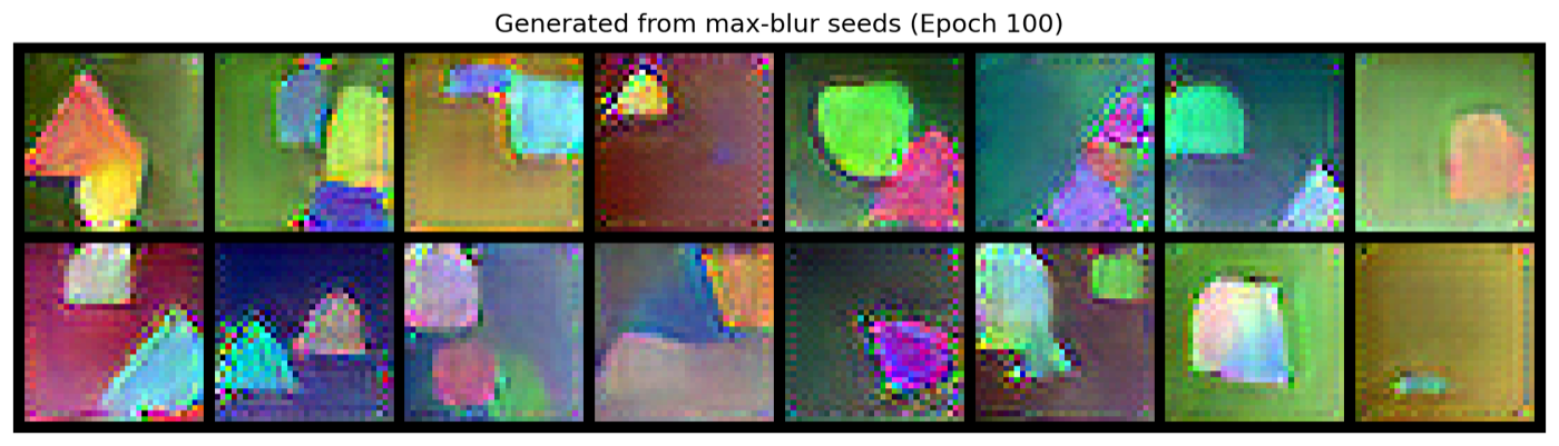
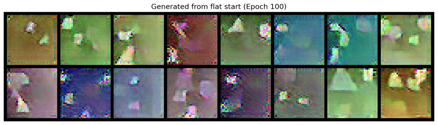
Reconstruction predicts u₀ in one shot; generation instead walks backward through the schedule — predict u₀, re-blur that prediction to t−1, feed it back in, and repeat down to t=0. Two starting points were tested: a real image blurred all the way to the maximum timestep, and a synthetic near-flat field with no information about any specific image at all.

Images generated by iteratively sharpening maximally-blurred versions of real images

Images generated by iteratively sharpening a near-uniform flat field with no seed image information

Left — generated by iteratively sharpening real images blurred to the maximum timestep: shapes and colors are largely recovered, close to the true seed. Right — generated from a near-uniform flat field with a small symmetry-breaking perturbation: the model still produces plausible blob-like shapes, but colors are muted and per-pixel speckle noise is visible — this is genuine synthesis, not reconstruction, and it shows.

The honest limitation

Because the forward process is deterministic, there is no built-in source of randomness to seed sample diversity the way Gaussian noise does in standard diffusion. Starting from a flat field with only a tiny random perturbation gives the reverse process very little to work with, and the result is visibly noisier and lower-fidelity than reconstruction from a real (if heavily blurred) image. This is a structural property of "cold" deterministic corruption processes, not a bug in this particular network — and it's the reason later work in this space (e.g. Cold Diffusion, Bansal et al. 2022) pairs a deterministic forward process with an explicit source of seed diversity.

Detail Builds Up Coarse-to-Fine

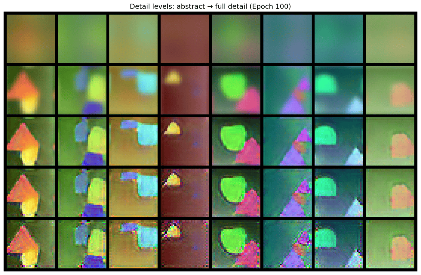
Stopping the reverse process early, at different timesteps, exposes the same coarse-to-fine hierarchy the forward process created — early stops give abstract color blobs, later stops progressively add shape and edge detail.

Grid showing the reverse process stopped at five different timesteps, from abstract flat colors to full detail

Same seeds, reverse process stopped at five points from most-blurred (top) to fully sharpened (bottom). Coarse color and rough shape appear first; fine edges and boundaries resolve last — the mirror image of how the forward process destroyed them.

Verifying the Physics: Mass Conservation and Frequency Decay

Two numerical checks confirm the forward process behaves exactly as the heat-equation math predicts.

Mass conservation

Total pixel intensity summed over the whole image, before and after blurring:

Blur level (t)	Original mass	Blurred mass	Ratio
0	1448.71	1448.71	1.0000
10	1448.71	1448.71	1.0000
15	1448.71	1448.71	1.0000
29 (max)	1448.71	1448.71	1.0000

Exact to the precision shown, at every blur level — the zero-frequency (DC) component is untouched by the Gaussian filter by construction, so total intensity can never drift.

High frequencies die first

Average FFT magnitude in five concentric frequency bands (band 1 = lowest frequencies, band 5 = highest), at increasing blur levels:

t	Band 1	Band 2	Band 3	Band 4	Band 5
0	19.66	3.03	1.63	1.17	0.99
5	19.66	3.03	1.63	1.17	0.99
10	19.64	3.00	1.59	1.11	0.91
15	19.44	2.70	1.20	0.65	0.39
29 (max)	7.40	0.00	0.00	0.00	0.00

By the final timestep, bands 2–5 have been destroyed completely (0.00), while band 1 (the lowest frequencies, closest to the mean color) still retains ~38% of its original energy — exactly the "fine detail dies first, coarse structure survives" hierarchy the forward process is designed to produce.

Extending to Real Datasets

Everything above trains on a small synthetic shapes dataset chosen for fast iteration and clean, interpretable structure. The repository also includes a more general, CLI-configurable version of the same method — a deeper U-Net with optional self-attention at low resolution, an optional stochastic perturbation during sampling, and out-of-the-box support for CIFAR-10, CIFAR-100, and CelebA. That script is provided as a documented starting point for scaling the method up; it has not yet been run to completion on a real photographic dataset, so no results are claimed for it here.